Model templates for Ontario
Patchworks uses the ForestModel language to describe stand dynamics. This language is complex and rich with features, providing power yet also making it a difficult system for casual users to master. One option that organizations can consider to make Patchworks model building easier for non-modelers is the use of model templates - an advanced and flexible data integration mechanism that is built into the baseline Patchworks product. Recently, Spatial Planning Systems worked with the Ontario Ministry of Natural Resources on a pilot project to explore using a model template for organizing forest management plan modeling data. In this article, we describe the implementation of this template.
Describing stand dynamics is a complex task in its own right and often represents a significant challenge for any modeling team. Although our knowledge of how stands grow is full of uncertainty, we model using deterministic notions that stands follow growth curves and respond to treatments in a predictable way. Modeling teams need to decide on and organize stratification schemes and develop growth and yield forecasts. There is an enormous amount of uncertainty in how elderly stands change – the senescence of older trees and the breakup and replacement of the canopy with a younger cohort – yet we capture this in simple rules for change that transitions occur at a given age. Silvicultural treatments in the virtual world must be coded symbolically, along with restrictions for what stand types are eligible for which actions, what costs and benefits flow from each treatment, and how each type will respond to form a future stand. Forest policy may require managing for special features, and these need to be characterized with indicators. Forests are complex, and the process of organizing, reviewing, and validating the descriptions of stand dynamics require an enormous amount of work.
ForestModel is a declarative XML (eXtensible Markup Language) language designed to specify how stand dynamics are modeled by the Patchworks system, including elements such as stratification variables, yield curves, succession, treatments, and responses. ForestModel contains many features and options that allow for building models that describe a wide range of forest conditions. Learning this language can be daunting for beginners due to of both the unfamiliar XML syntax and the large library of functions available in the query language. The staff specialists who prepare the stand dynamics information may not have the time or inclination to learn an arcane modeling language.
Model templates divide the model-building complexity into two parts:
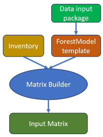
The inputs to the model – inventory, stratification variables, yield curves, succession, treatments, responses, indicators, etc. – are organized into a set of related tables. The semantics of these tables are well defined: the tables have agreed-upon standard names with agreed-upon columns headings, and the contents have specific meanings. We will refer to this set of related tables as the data input package.
The templating features of the ForestModel language are used to write a ForestModel XML file that will read the tables from the data input package and introspect on the inventory and yield curve datasets to adapt to the values that have been provided. We will refer to this ForestModel XML file as the model template.
Together, the data input package and the model template can be used to build a Patchworks input dataset.
With this division of the problem, the staff specialists who are familiar with the local forest can learn the language of the data input package and populate these tables with values appropriate to their situation, with no need to learn the specifics of the XML language.
The model template file must be developed by an expert in the ForestModel language. The template will contain the logic of how the stand dynamics will be applied, but it will be empty of the local forest data values. When the template is run, it will load the relationships from a specified data input package and configure itself to render values for that forest. The ForestModel template needs to be developed once and can then be copied and applied as-is to any standard data input package.
The next sections will briefly describe some of the tables in the Ontario data input package and some of the templating features in the companion ForestModel. At the end of this article are links to the Ontario ForestModel template file and several example data input packages. While this template is specific to the Ontario situation, it can serve as a useful "how to" for those considering building templates for their own modeling problems.
The rest of this article is a blend of high-level overview and nerdy detail. For those who just want to get a general idea of how the template works, feel free to skip over the technical bits. If you are already familiar with Patchworks and the ForestModel and really want to understand the implementation, then as you read through the following explanations, you may want to refer to the ForestModel documentation to get a more thorough explanation of the elements and options. The Patchworks Query Language documentation will help to explain the expressions that are used to define fields, calculate curve values, and select records.
Design criteria
Ontario has 27.8 million hectares of managed forest spanning from the Great Lakes-St Lawrence region to the Boreal. Along with the geographic range of these forests comes a diversity of ecological, silvicultural, operational, and policy issues. One of the objectives of the pilot project was to examine the commonality of concerns and determine if a single model template could meet the needs of the Northwestern, Northeastern, and Southern regions. One of the differences is that the Northwest region and most of the Northeast region only apply even-aged silviculture, while the Southern region and a few units in the Northeast region also apply shelterwood and selection silviculture. The northern regions apply the boreal landscape guide, while the Southern region applies the GLSL landscape guide. The Northwest and Southern regions use a 1:1 deterministic approach to post-treatment and post-successional responses, while the Northeast region is pursuing a proportional-response-based approach.
The fortunate outcome of this pilot project is that the model template accomplishes this goal, albeit at the small expense of slightly more complicated coding in the ForestModel XML template. The template only generates outcomes for values entered into the data input package. If there are no entries in the shelterwood and selection tables, then none of these treatment types will be generated. The two landscape guides have a similar enough structure that the same template components can be used for both. The proportional-response method requires a few extra columns of of information, and the template will detect their presense and configure itself accordingly.
A walk through of the data input package and template
The data input package is a collection of related tables in a standard format. Patchworks can access tabular data in a wide variety of formats, but for the Ontario template, we have chosen to use Excel workbooks as the container for our tables. Although Excel is not as robust as enterprise solutions such as Postgres, it is ubiquitous, familiar to most, easy to work with, and easy to share, providing a low barrier to entry for forest specialists who are not IT specialists.
The organization of the Excel data input package consists of a series of sheets, each having a standard name and organization of rows and columns. Many of the input tables identified in the pilot project bear a strong similarity to the input tables of the predecessor Ontario SFMM model, which is not unexpected since the fundamental modeling paradigm has not changed much.
| Table Name | Purpose |
|---|---|
| Notes | This table provides a space to log changes to the input package, but is not otherwise used by the model. |
| YieldTables | Describe the file names and formatting of the yield tables |
| InputColumns | Identify the input source for stratification variables |
| GenericSpecies | Provide a mapping from inventoried species to generic species (e.g. from multiple poplar species to simply Po) to reduce the number of components in the model |
| NaturalSuccession | Rules for stand breakup and renewal |
| CC_Treatments | Rules for even-aged treatments and post-treatment conditions |
| CC_Operability | Rules for even-aged treatment eligibility |
| UnharvestedVolume | Volume reduction factors for bypass and non-commercial species, by treatment type and species |
| SH_Treatments | Rules for shelterwood treatments and post-treatment conditions |
| SE_Treatments | Rules for selection harvest treatments and post-treatment conditions |
| Products | Product definitions and renewal charges |
| LGC definitions | Landscape guide classifications |
| LGC targets | Targets for landscape guides |
| LLP Definitions | Definitions for large landscape patches features |
| LLP_Targets | Targets for large landscape patches |
| Biological limits | Production limits on the biological capacity of the forest |
| Operational Limits | Capacity limits on production |
| TreesPlanted | Seedling requirements by treatment type |
| RoadsLandingsWSY | Areas removed from production by roads and landings |
| HarvestPatches | Harvest patch size categories |
| MIllRequirements | Mill quotas by product types |
The general design of the data input workbook is that the table data always begins with the column headings in row four of each sheet. The previous three rows of each sheet are ignored and may contain supplemental headings and instructions. Excel formatting (fonts, background cell colours, cell borders, etc.) is ignored and may be customized as desired. Cell comments and other objects (text boxes, arrows, lines, and other shapes) are ignored and can be used to highlight model features.
As the MatrixBuilder application loads the template, it will read the tables in the data input package and install them as lookup tables in the modeling environment. Each table can be referred to in subsequent queries by its sheet name. The following sections will walk through a few of the tables in the data input package and explain how these are used in the template model.
Notes
There is not much to say about this table, other than it is a free-form space to record changes that have been made to the data inputs. The value of this table is for future modelers to read about the sequence of modifications and the justification for the changes. The model template does not reference this table in any way.

YieldTables
The YieldTables table contains one row for each distinct yield file that is to be read in. Yield tables are read with the ForestModel curvetable element, which has the flexibility to read many different yield file formats. The table contains four columns:
- FILE
The name of the yield curve file, as a relative path from the location of the data package. The file is expected to contain tabular data with column headings and rows (such as a CSV file, dBase file, Excel sheet reference) or be a query on a DBMS that returns a row set.
- AGE
The name of the column in the yield curve table that contains the age value for each record.
- Label
An expression that will compute a label for each curve that is being read in. Similar to the title of a book, the label is the unique identifier that is used to store and retrieve the curves from the library. The expression contains a combination of literal strings and cell values from the yield curve file.
- IgnoreColumns
A list of columns contained in the yield file that are superfluous, such as species composition.
An example of a YieldCurve table is as follows, which contains rows for stand-level curves, strata-level curves, and product proportions:

Click image to enlarge
This table contains three rows of curve table references: one for stand-based curves, one for strata-based curves, and one that describes how product proportions change over time. Stand-level curves are based on detailed inventory characteristics from the recent lidar-based inventory and are used for the first rotation. Strata-level curves are developed in the usual way and are applied to second rotation and post-successional stands where the detailed stand observations are no longer available.
The label expressions vary in each row of the 'YieldCurves' table. For the first row that describes the stand-level curves, each curve can be uniquely defined by the stand id and the species code. The label expression ('Stand:'+ID+':%h') begins with the literal 'Stand:' followed by the unique id for the polygon, followed by the literal ':%h'. This final string contains the special '%h' column heading substitution symbol. When the curve file is read, the values from the columns that contain the species volumes will be extracted into curves, and the '%h' in the label expression will be replaced with the column heading from which curve originates.
The strata-level curves are stratified by forest unit, timber capability rating, acceptable growing stock fraction, and a yield intensity classification, as seen in the label expression ( 'Strata:'+yFU+':'+TCR+':'+AGSFRC+':'+YIELD+':%h'). This expression begins with the literal 'Strata:' to easily distinguish strata-level from stand-level curves.
The IgnoreColumns value provides a list of columns in the yield curve table that should not be converted into yield curves. For the most part, these columns contain additional stratification values, such as species composition or leading species.
The code in the model template that processes this table uses a loop to iterate over each row in the table:
<repeat name="y" table="YieldTables">
  <curvetable file="getEnv('repeat.y.FILE')" ageexpression="eval(getEnv('repeat.y.AGE'))" patternexpression="eval(getEnv('repeat.y.Label'))" ignorecolumns="getEnv('repeat.y.IgnoreColumns')" missing="NA" replacemissing="0">
  </curvetable>
</repeat>
During each pass through the loop, the values from the current row of the YieldCurves table are set to a repeat variable that is prefixed with the letter y. The curvetable element is executed each time through the loop, substituting in command options from the columns of the table.
The end result is that curves are read from each file listed in the table. As curves are read, they are entered into an internal curve library. In a later section, we will see how these curves are retrieved from the library and attached to the stand dynamics descriptions for each polygon.
InputColumns
This table contains a mapping between the symbolic variable names used in the template and the actual columns that exist in the inventory. Although the inventory datasets used for forest management plan modeling in Ontario have some standardization, there is room for variability, and in practice, no two files seem to be formatted in the exact same way.
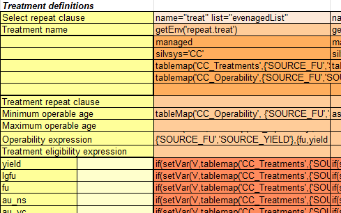
There are two main sets of input column mappings that are required: one for basic polygon information (shown with a yellow-tan background in the table below), and the other for stratification columns (shown with an orange background in the table below). Basic polygon information includes the unique name for each inventory unit, the area of each inventory unit, and a query to determine if the polygon is included or excluded from the analysis. Stratification values include the symbolic name used internally in the template and an expression applied to the row of the inventory to calculate the stratification value. This template model for Ontario always uses the same number of stratification variables with the same symbolic names, but of course, the stratification values themselves will be read from the inventory data.
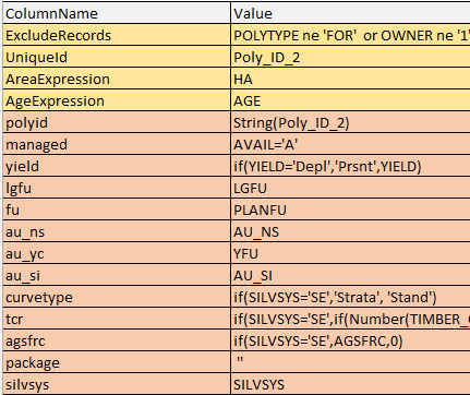
For many stratification variables, the expression is simply the name of the inventory column that contains the value, but in other cases, a transformation may be used, for example, to handle missing or wrongly coded values.
In the above example, the managed stratification variable expects a boolean true/false value, and the expression compares the value of the AVAIL inventory column to the code 'A' for available. The data input package is not expecting the yield code of 'Depl', so this value that is present in the BMI is recoded on the fly to 'Prsnt'. As can be seen in the figure, the stratification system includes several different analysis units: the landscape guide forest unit, the forest unit, the natural succession analysis unit, the post-treatment analysis unit, etc. The initial type of yield curve to use is the stand level curves, except for selection silviculture, where the strata curves have higher reliability, and so on. Each of these stratification variables influences the matching of rules in the template as the MatrixBuilder works through the stands one by one.
The template code for the input columns appears as follows:
  <input block="eval(tableMap('InputColumns','ColumnName','UniqueId','Value'))" area="eval(tableMap('InputColumns','ColumnName','AreaExpression','Value'))" age="eval(tableMap('InputColumns','ColumnName','AgeExpression','Value'))" exclude="eval(tableMap('InputColumns','ColumnName','ExcludeRecords','Value'))"  />

  <define field="polyid" column="eval(tableMap('InputColumns','ColumnName','polyid','Value'))" />
  <define field="managed" column="eval(tableMap('InputColumns','ColumnName','managed','Value'))" />
  <define field="yield" column="eval(tableMap('InputColumns','ColumnName','yield','Value'))" />
  <define field="lgfu" column="eval(tableMap('InputColumns','ColumnName','lgfu','Value'))" />
  <define field="fu" column="eval(tableMap('InputColumns','ColumnName','fu','Value'))" />
  <define field="au_ns" column="eval(tableMap('InputColumns','ColumnName','au_ns','Value'))" />
  <define field="au_si" column="eval(tableMap('InputColumns','ColumnName','au_si','Value'))" />
  <define field="au_yc" column="eval(tableMap('InputColumns','ColumnName','au_yc','Value'))" />
  <define field="curvetype" column="eval(tableMap('InputColumns','ColumnName','curvetype','Value'))" />
  <define field="tcr" column="eval(tableMap('InputColumns','ColumnName','tcr','Value'))" />
  <define field="agsfrc" column="eval(tableMap('InputColumns','ColumnName','agsfrc','Value'))" />
  <define field="package" column="eval(tableMap('InputColumns','ColumnName','package','Value'))" />
  <define field="silvsys" column="eval(tableMap('InputColumns','ColumnName','silvsys','Value'))" />
In the above lines, the tablemap function retrieves the cell contents from the data input package, and the eval function compiles the results into expressions that can be applied to each input record. Although the above statements may seem repetitive and verbose, this method isolates the values that change with each forest from the template. The template doesn't change; it just needs to point to a different data input package.
GenericSpecies
This table lists all the species encountered in the growth and yield files and recodes some of the names into 'generic species' coding. The purpose of this recoding is that the Great Lakes-St Lawrence forest contains many minor species, to the extent that indicators and summaries would be cluttered if all were represented. The generic species recoding collapses minor species into a simpler generic code. For example, in a sample Great Lakes-St Lawrence forest, black ash, white ash, basswood, black cherry, elm, ironwood, and Manitoba or striped maple are relatively non-commercial minor species that are recoded to OH (other hardwoods).
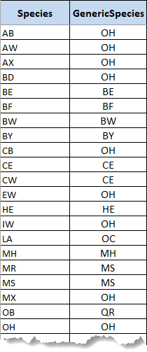
As the template attaches volumes to stands, the recoding will be used to aggregate the detailed species into generic species curves. Elsewhere in the model, only the generic species codes are used. To make this compression from detailed species to generic species, the template will first transform the GenericSpecies table into lists of all of the minor species associated with each generic species.
<define field="standSppList" constant="listremove(sort(unique(filter(curveNames(),'Stand:.*\:(\w*)','{1}'))),{'DBHQ','STEMS','HT','BA','GTV','GMV','NMV'})" />
<define field="strataSppList" constant="listremove(sort(unique(filter(curveNames(),'Strata:.*\:(\w*)','{1}'))),{'DBHQ','STEMS','HT','BA','GTV','GMV','NMV'})" />
<define field="genericSpp" constant="sort(unique(tablelist('GenericSpecies','GenericSpecies')))" />
<repeat name="g" list="genericSpp">
  <define field=" 'generic_stand_'+getEnv('repeat.g')" constant="asList(tablelist('GenericSpecies','Species',q($getEnv('repeat.g')=GenericSpecies and Species in '$)+join(standSppList,',')+q($'$)),{''})" />
</repeat>
<repeat name="g" list="genericSpp">
  <define field=" 'generic_strata_'+getEnv('repeat.g')" constant="asList(tablelist('GenericSpecies','Species',q($getEnv('repeat.g')=GenericSpecies and Species in '$)+join(strataSppList,',')+q($'$)),{''})" />
</repeat>
These queries introspect the names of the curves that have been read into the curve library to determine what species are actually present in the yield data, and then collate the values into lists of detailed species for each generic species. The expressions that calculate the lists may seem complicated at first, but are quite simple when broken down into smaller steps. For example, the standSppList expression includes the following steps:
Get a list of the names of all curves in the library.
Filter the list to include only curve names that start with 'Stand:' and extract the last component of the curve name (the species code).
Reduce this list to only include unique names and sort them in alphabetic order.
Remove the curve names that are not species (DBHQ, STEMS, HT, BA, GTV, GMV, NMV).
The expression for the strataSppList is similar to the above, changing the filtering criteria to yield curve names that start with 'Strata:'.
The expression for the genericSpp list is very simple:
Make a list from the values in the 'GenericSpecies' column in the 'GenericSpecies' table.
Reduce this list to unique values and sort.
The lists of detailed species for each generic species are created using a repeat loop. There is a set of lists for species found in the stand yield curves and another set of lists for species found in the strata yield curves, produced as follows:
Loop over a define element that will create a list for each generic species code.
Calculate the name of the list by concatenating 'generic_stand_' with the generic species code for this loop iteration.
Use the tablelist function to obtain a list from the 'Species' column of the 'GenericSpecies' table for the rows where the GenericSpecies column matches the generic species code that we are looping over, and where the species code is found in the stand species list.
The following shows the lists resulting from executing the above ForestModel code on a sample Great Lakes-St Lawrence forest. You can see that the strata-based curves contain more species columns than the stand-based curves:
define constant standSppList:  {'AB', 'BE', 'BF', 'BW', 'BY', 'CE', 'HE', 'LA', 'MH', 'MS', 'OH', 'OR', 'PJ', 'PO', 'PR', 'PW', 'SB', 'SW'}
define constant strataSppList:  {'AB', 'AW', 'AX', 'BD', 'BE', 'BF', 'BW', 'BY', 'CB', 'CE', 'CW', 'EW', 'HE', 'IW', 'LA', 'MH', 'MR', 'MS', 'MX', 'OB', 'OH', 'OR', 'OW', 'PB', 'PJ', 'PL', 'PO', 'PR', 'PS', 'PT', 'PW', 'SB', 'SN', 'SR', 'SW', 'SX'}
define constant genericSpp:  {'BE', 'BF', 'BW', 'BY', 'CE', 'HE', 'MH', 'MS', 'OC', 'OH', 'PJ', 'PO', 'PR', 'PW', 'QR', 'SB', 'SW'}
define constant generic_stand_BE:  {'BE'}
define constant generic_stand_BF:  {'BF'}
define constant generic_stand_BW:  {'BW'}
define constant generic_stand_BY:  {'BY'}
define constant generic_stand_CE:  {'CE'}
define constant generic_stand_HE:  {'HE'}
define constant generic_stand_MH:  {'MH'}
define constant generic_stand_MS:  {'MS'}
define constant generic_stand_OC:  {'LA'}
define constant generic_stand_OH:  {'AB', 'OH'}
define constant generic_stand_PJ:  {'PJ'}
define constant generic_stand_PO:  {'PO'}
define constant generic_stand_PR:  {'PR'}
define constant generic_stand_PW:  {'PW'}
define constant generic_stand_QR:  {'OR'}
define constant generic_stand_SB:  {'SB'}
define constant generic_stand_SW:  {'SW'}
define constant generic_strata_BE:  {'BE'}
define constant generic_strata_BF:  {'BF'}
define constant generic_strata_BW:  {'BW'}
define constant generic_strata_BY:  {'BY'}
define constant generic_strata_CE:  {'CE', 'CW'}
define constant generic_strata_HE:  {'HE'}
define constant generic_strata_MH:  {'MH'}
define constant generic_strata_MS:  {'MR', 'MS'}
define constant generic_strata_OC:  {'LA', 'PS'}
define constant generic_strata_OH:  {'AB', 'AW', 'AX', 'BD', 'CB', 'EW', 'IW', 'MX', 'OH'}
define constant generic_strata_PJ:  {'PJ'}
define constant generic_strata_PO:  {'PB', 'PL', 'PO', 'PT'}
define constant generic_strata_PR:  {'PR'}
define constant generic_strata_PW:  {'PW'}
define constant generic_strata_QR:  {'OB', 'OR', 'OW'}
define constant generic_strata_SB:  {'SB'}
define constant generic_strata_SW:  {'SN', 'SR', 'SW', 'SX'}
Later in the ForestModel codes like the one below are used to sum all of the minor species growing stock volumes by generic species. This particular code will attach the computed stand attribute curve to the polygon condition currently under consideration. In this case, the select clause only applies the enclosed elements when the curvetype is 'Stand', normally during the first rotation. After the first rotation, or the first successional event, the curvetype stratification variable will be changed to 'Strata', and a different code will be selected.
  <select statement="curvetype='Stand'">
    <features>
     <repeat name="genspp" list="genericSpp">
      <attribute label=" '%f.Yield.%m.'+getEnv('repeat.genspp')" factor="1-asNumber(tableMap('RoadsLandingsWSY','SOURCE_FU',fu,yield))" output="nonzero">
        <expression statement="asCurve(eval(join(filter(eval('generic_stand_'+getEnv('repeat.genspp')),'.*',q($curvematch(':','Stand',polyid,'{0}')$)),'+')))" by="1" ignoreMissingAttributes="false"/>
      </attribute>
     </repeat>
    </features>
  </select>
In the above code, the repeat loop iterates over the list of generic species, so there will be one yield curve attached for each generic species. The attribute label (the name given to the attached yield curve) is computed from an expression based on the value of the repeat loop. In addition, the curve value is reduced by a scaling factor obtained by looking up the value from the 'RoadsLandingsWSY' table.
As you can see, the query code can be quite inscrutable for these complex summations. The expression statement uses a filter function to iterate over the list of detailed species for each generic species. Each of the detailed species codes is interpolated into a curvematch query (to look up values with wildcard alternatives), and the query fragments are joined together with addition operators. Note that this expression applies to stand-level curves, and the parameters to the curvematch function include the string 'Stand' as well as the polygon ID and the species code.
After executing the repeat loops and expressions, the resulting code expands to the following:
<select statement="curvetype='Stand'">
  <features>
    <attribute label="'%f.Yield.%m.OH'" factor="1-asNumber(tableMap('RoadsLandingsWSY','SOURCE_FU',fu,yield))" output="nonzero">
      <expression statement="curvematch(':','Stand',polyid,'AB')+ curvematch(':','Stand',polyid,'OH')" )))" by="1" ignoreMissingAttributes="false"/>
   </attribute>
  </feature>
</select>
The MatrixBuilder application will test and apply this pattern to each polygon for their current stratification values, attaching the yield curves when the selection criteria match. The MatrixBuilder recursively steps through treatments and then post-treatment conditions (as well as succession and post-succession conditions), and will again test and apply the entire set of patterns based on the future stratification values.
Although complex, these expressions need only to be composed once by a specialist modeler. After being debugged and verified, they can then be applied to any data input package.
Natural Succession
The natural succession table is more complex in terms of entries but perhaps easier to understand. The table is made up of two sets of columns: the current conditions and the future conditions.
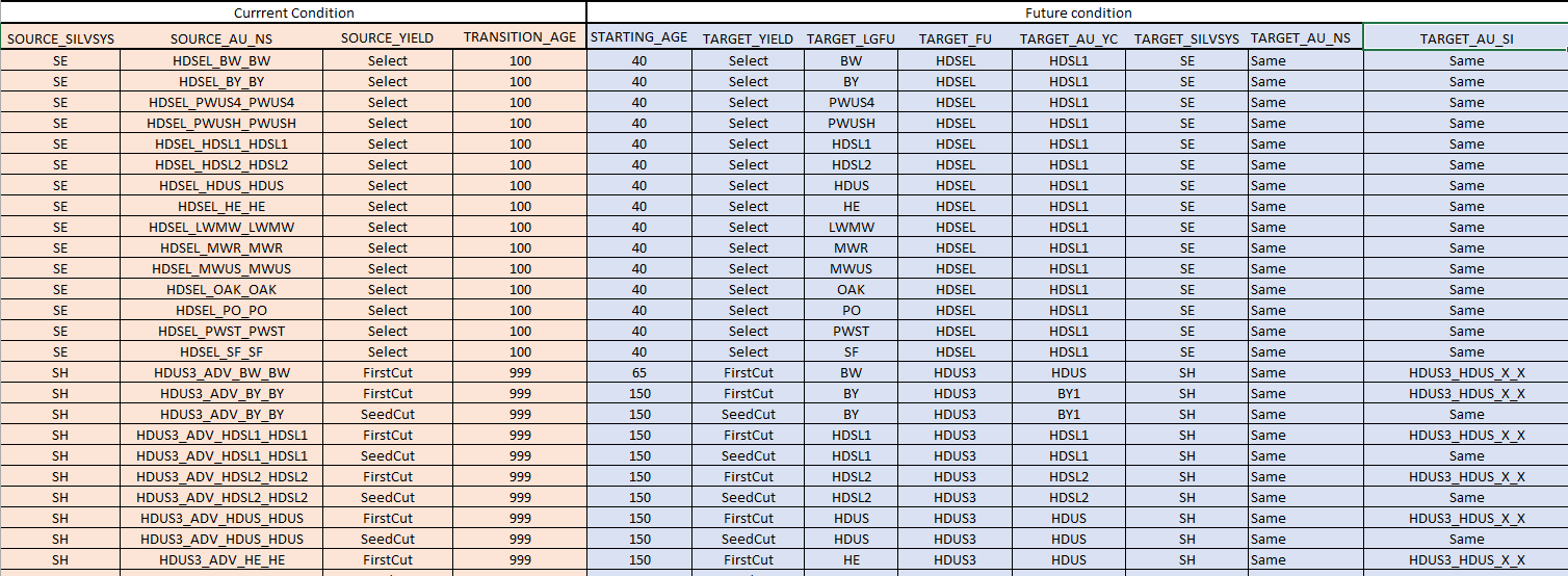
Click image to enlarge
Stands that match the current conditions at the transition age will have their stratification values changed to the future conditions, with the age reset to the new starting age. The template ForestModel code to implement these transitions is:
<select>
    <succession breakup="Number(tablemap('NaturalSuccession',{'SOURCE_SILVSYS','SOURCE_AU_NS','SOURCE_YIELD'},{silvsys,au_ns,yield},'TRANSITION_AGE',999))" renew="Number(tablemap('NaturalSuccession',{'SOURCE_SILVSYS','SOURCE_AU_NS','SOURCE_YIELD'},{silvsys,au_ns,yield},'STARTING_AGE',100))" >
      <assign field="yield" value="if(setVar('v',tablemap('NaturalSuccession',{'SOURCE_SILVSYS','SOURCE_AU_NS','SOURCE_YIELD'},{silvsys,au_ns,yield},'TARGET_YIELD'))='Same',yield,getVar('v'))"/>
      <assign field="lgfu" value="if(setVar('v',tablemap('NaturalSuccession',{'SOURCE_SILVSYS','SOURCE_AU_NS','SOURCE_YIELD'},{silvsys,au_ns,yield},'TARGET_LGFU'))='Same',lgfu,getVar('v'))"/>
      <assign field="fu" value="if(setVar('v',tablemap('NaturalSuccession',{'SOURCE_SILVSYS','SOURCE_AU_NS','SOURCE_YIELD'},{silvsys,au_ns,yield},'TARGET_FU'))='Same',fu,getVar('v'))"/>
      <assign field="au_ns" value="if(setVar('auns',tablemap('NaturalSuccession',{'SOURCE_SILVSYS','SOURCE_AU_NS','SOURCE_YIELD'},{silvsys,au_ns,yield},'TARGET_AU_NS'))='Same',au_ns,getVar('auns'))"/>
      <assign field="au_yc" value="if(setVar('v',tablemap('NaturalSuccession',{'SOURCE_SILVSYS','SOURCE_AU_NS','SOURCE_YIELD'},{silvsys,au_ns,yield},'TARGET_AU_YC'))='Same',au_yc,getVar('v'))"/>
      <assign field="au_si" value="if(setVar('v',tablemap('NaturalSuccession',{'SOURCE_SILVSYS','SOURCE_AU_NS','SOURCE_YIELD'},{silvsys,au_ns,yield},'TARGET_AU_SI'))='Same',au_si,getVar('v'))"/>
     <repeat name="r" list="respList">
      <assign field=" 'Resp_'+getEnv('repeat.r')" value="tablemap('NaturalSuccession',{'SOURCE_SILVSYS','SOURCE_AU_NS','SOURCE_YIELD'},{silvsys,au_ns,yield},'TARGET_FU')+'_Future'"/>
     </repeat>
      <assign field="curvetype" value="'Strata'"/>
      <assign field="polyid" value="'0'"/>
    </succession>
  </select>
Note that the breakup and renewal ages are looked up in the NaturalSuccession table by a combination of silvicultural system, natural selection analysis unit, and current yield condition codes. Similarly, all of the assignments of the new target codes are also looked up in the table. The one variation to be noted here is that if the target code is 'Same', then the value will stay the same (it will be assigned the current value). The following pseudo-code outlines the logic of the yield assignment statement:
v = Lookup the 'TARGET_YIELD' value from the 'NaturalSuccession' table by silvsys, au_ns, and yield
if v equals 'Same'
   yield = yield
else
   yield = v
The model template code is verbose and repetitive, but again, it only needs to be developed and verified once.
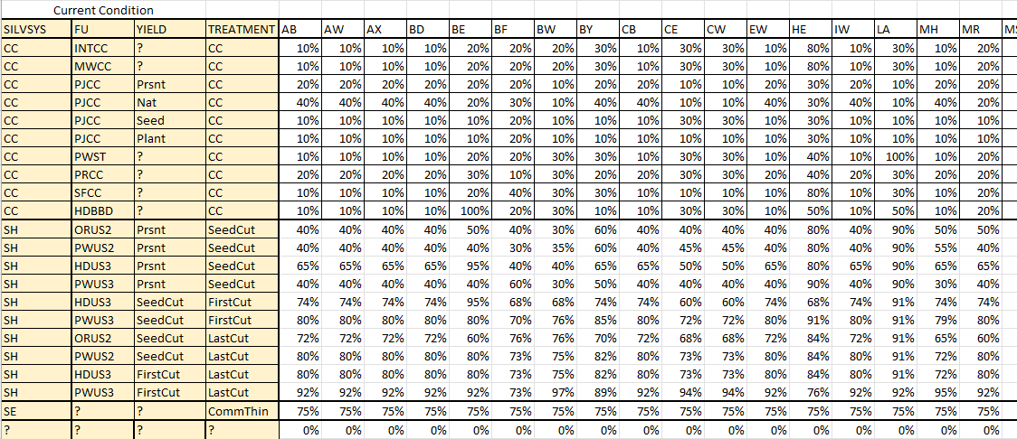
CC_Treatments
The CC_Treatments table is similar to the NaturalSuccession table, containing the current conditions that must be matched and the future conditions that will be updated if the treatment is chosen. In addition to the current and future conditions for the stratification variables, the table also includes the name of the treatment and the cost per hectare for the renewal treatment. In this model, harvest and treatment options are linked: choosing a treatment implies both the harvest event and the immediately following silvicultural treatment. It is possible to decouple harvest and renewal into two separate events, but for this model formulation, it is unnecessary.

Click image to enlarge
The template code for even-aged treatments and responses is shown below. This code is getting a bit longer, but most of it consists of the repetitive code that updates the stratification variables to their post-treatment conditions.
<repeat name="treat" list="evenagedList">
  <select statement="managed and silvsys='CC' and tablemap('CC_Treatments',{'SOURCE_FU','SOURCE_AU_SI','TREATMENT'},{fu, if(listsize(respList)>0,column('Resp_'+getEnv('repeat.treat')), au_si), getEnv('repeat.treat')},'TREATMENT','') ne '' and tablemap('CC_Operability',{'SOURCE_FU','SOURCE_YIELD'},{fu,yield},'MIN_AGE',-1) ne -1">
    <track>
      <treatment label="getEnv('repeat.treat')" minage="tableMap('CC_Operability', {'SOURCE_FU','SOURCE_YIELD'},{fu,yield},'MIN_AGE')" operability="setVar('minv',tableMap('CC_Operability', {'SOURCE_FU','SOURCE_YIELD'},{fu,yield},'MIN_VOLUME','')); setVar('spg',tableMap('CC_Operability', {'SOURCE_FU','SOURCE_YIELD'},{fu,yield},'SPECIES_GROUP','')); if(getVar('minv')='',true,lookupCurve(attribute(if(getVar('spg')='','feature.total.Yield.managed','feature.YieldSpg.managed.'+getVar('spg'))),offset()) ge Number(getVar('minv')))">
        <produce>
          <assign field="treatment" value="getEnv('repeat.treat')"/>
          <assign field="action" value="getEnv('repeat.treat')"/>
          <assign field="next_yield" value="if(setVar('v',tablemap('CC_Treatments',{'SOURCE_FU','SOURCE_AU_SI','TREATMENT'},{fu,if(listsize(respList)>0,column('Resp_'+getEnv('repeat.treat')), au_si),getEnv('repeat.treat')},'TARGET_YIELD'))='Same',yield,getVar('v'))"/>
        </produce>
        <transition>
          <assign field="yield" value="if(setVar('v',tablemap('CC_Treatments',{'SOURCE_FU','SOURCE_AU_SI','TREATMENT'},{fu,if(listsize(respList)>0,column('Resp_'+getEnv('repeat.treat')), au_si),getEnv('repeat.treat')},'TARGET_YIELD'))='Same',yield,getVar('v'))"/>
          <assign field="lgfu" value="if(setVar('v',tablemap('CC_Treatments',{'SOURCE_FU','SOURCE_AU_SI','TREATMENT'},{fu,if(listsize(respList)>0,column('Resp_'+getEnv('repeat.treat')), au_si),getEnv('repeat.treat')},'TARGET_LGFU'))='Same',lgfu,getVar('v'))"/>
          <assign field="fu" value="if(setVar('v',tablemap('CC_Treatments',{'SOURCE_FU','SOURCE_AU_SI','TREATMENT'},{fu,if(listsize(respList)>0,column('Resp_'+getEnv('repeat.treat')), au_si),getEnv('repeat.treat')},'TARGET_FU'))='Same',fu,getVar('v'))"/>
          <assign field="au_ns" value="if(setVar('v',tablemap('CC_Treatments',{'SOURCE_FU','SOURCE_AU_SI','TREATMENT'},{fu,if(listsize(respList)>0,column('Resp_'+getEnv('repeat.treat')), au_si),getEnv('repeat.treat')},'TARGET_AU_NS'))='Same',au_ns,getVar('v'))"/>
          <assign field="au_yc" value="if(setVar('v',tablemap('CC_Treatments',{'SOURCE_FU','SOURCE_AU_SI','TREATMENT'},{fu,if(listsize(respList)>0,column('Resp_'+getEnv('repeat.treat')), au_si),getEnv('repeat.treat')},'TARGET_AU_YC'))='Same',au_yc,getVar('v'))"/>
          <assign field="au_si" value="if(setVar('v',tablemap('CC_Treatments',{'SOURCE_FU','SOURCE_AU_SI','TREATMENT'},{fu,if(listsize(respList)>0,column('Resp_'+getEnv('repeat.treat')), au_si),getEnv('repeat.treat')},'TARGET_AU_SI'))='Same',au_si,getVar('v'))"/>
          <assign field="package" value="''"/>
         <repeat name="r" list="respList">
          <assign field="'Resp_'+getEnv('repeat.r')" value="tablemap('CC_Treatments',{'SOURCE_FU','SOURCE_AU_SI','TREATMENT'},{fu,column('Resp_'+getEnv('repeat.treat')),getEnv('repeat.treat')},'TARGET_FU','')+'_Future'"/>
         </repeat>
          <assign field="inPackage" value="false"/>
          <assign field="curvetype" value="'Strata'"/>
          <assign field="polyid" value="'0'"/>
        </transition>
      </treatment>
    </track>
  </select>
 </repeat>
The first element of the code is a repeat loop that iterates through all the names of the even-aged treatments. The second element is a selection clause that tests if the polygon conditions match the expression. In this case, the expression tests whether the polygon is eligible for treatments (with the managed boolean being true), in the CC silvicultural system, has a record in the CC_Treatments table that matches the current fu, yield and au_si stratification columns, and that there is an entry for the current condition in the CC_Operability table. If all of these conditions are met, the treatment option will be attached to the current condition as a candidate.
The test for having a matching row in the CC_Treatments table is slightly complicated because there is a test to see if proportional allocation is used. If so, additional response columns are tested for a non-blank value.
The treatment element defines the treatment name (taken from the repeat variable), the minimum operable age (from the CC_Operability lookup table), and an optional minimum volume operability expression.
The remainder of this code updates the stratification variables to their post-treatment condition, similar to the method described previously for the NaturalSuccession table.
After the MatrixBuilder determines the candidate treatments for the current condition, it will recursively update the stratification variables and repeat the process of attaching yield curves and determining candidate treatments for the next rotation, and so on until the forecast is far enough into the future to exceed the planning horizon.
The SH_Treatments (shelterwood) and SE_Treatments (selection) tables are similar in concept but follow different prescribed treatment sequences.
UnharvestedVolume
The UnharvestedVolume table describes the amount of standing volume that does not contribute to wood supply when a treatment is selected. Volume may be left unharvested for a number of reasons, for example, the lack of a commercial market for the species or to achieve conservation objectives.
Click image to enlarge
This table has a set of columns that must match the current condition and columns of the original detailed species codes. The cells under the species codes contain the unharvested reduction factor.
The following template code shows the unharvested deductions being applied.
  <select statement="silvsys in 'CC,SH,SE' and curvetype='Stand'">
    <products>
     <repeat name="genspp" list="genericSpp">
      <attribute label=" 'tempStandHarvest.'+getEnv('repeat.genspp')" output="false">
        <expression statement="asCurve(eval(join(filter(eval('generic_stand_'+getEnv('repeat.genspp')),'.*',q($(curvematch(':','Stand',polyid,'{0}')*(1-tablemap('UnharvestedVolume',{'FU','YIELD','TREATMENT'},{fu,yield,treatment},{0},0)))$)),'+')))" by="1" ignoreMissingAttributes="false"/>
      </attribute>
     </repeat>
    </products>
  </select>
This is similar to the code shown previously that used the GenericSpecies table to calculate growing stock, except that the unharvested volume deductions are applied.
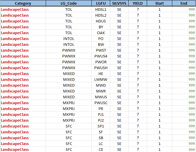
LGC definitions
The LGC definitions table contains the criteria for the landscape guide classifications. The first two columns describe the landscape guide category and code that the row applies to. The LGFU, SILVSYS, and YIELD columns are stratification values that must match the corresponding stratification variables. Finally, the Start and End columns describe the range of ages for which the landscape indicator is active.
The template code for this section is concise:
<repeat name="lg" table="LGC definitions">
  <select statement="((silvsys = getEnv('repeat.lg.SILVSYS') or '?' =  getEnv('repeat.lg.SILVSYS')) and (lgfu = getEnv('repeat.lg.LGFU') or '?' =  getEnv('repeat.lg.LGFU')) and (yield = getEnv('repeat.lg.YIELD') or '?' = getEnv('repeat.lg.YIELD')))">
    <features>
      <attribute label=" '%f.LG.'+getEnv('repeat.lg.Category')+'.'+getEnv('repeat.lg.LG_Code')" factor="1-asNumber(tableMap('RoadsLandingsWSY','SOURCE_FU',fu,yield))" output="nonzero">
        <expression statement="curveClip(curve(0,1,999,1),Number(getEnv('repeat.lg.Start')),Number(getEnv('repeat.lg.End')))" by="1" ignoreMissingAttributes="false"/>
      </attribute>
    </features>
  </select>
 </repeat>
The outer element loops through each of the rows in the LGC definitions table. The selection clause restricts matches to those records where the LGFU, SILVSYS, and YIELD columns match the corresponding stratification values or where the value is a wildcard '?'. The attribute name is calculated from the Category and LG_Code values for the matching row, and the shape of the curve is computed from the Start and End values.
The Biological Limits and Operational Limits tables are handled in a similar manner.
Choosing the data input package
The model template has been designed so that one template can work unchanged with any compatible data input package. But how does the template know what data input package to process?
The ForestModel language has an <exec> element that allows running an external script, and the model template makes use of this to prompt for the data input package file name:
<exec interpreter="beanshell">
  <script><![CDATA[
  {
    /*
     * Query for the data input package
     */

    // Check if input package name already specified (batch mode)
    dataInputPackage = System.getProperty("dataInputPackage");
    if (dataInputPackage != null) {
        if(new File(dataInputPackage).exists())
            return;
        else
            throw new IllegalStateException("File "+dataInputPackage+" not found");
    }

    // Initialize the file chooser
    SFileFetch sff = new SFileFetch("Data Input Package");
    sff.addFilter(new String[]{"xlsx","xlsm","xlsb"}, "Excel workbook");
    sff.setMatchingFilter(new File("temp.xlsx"));

    // Get the saved value if available
    Properties props = IProperties.loadProps();
    dataInputPackage = props.getProperty("builder.dataInputPackage", "");

    // Determine the initial folder - either the saved input file or the location of the XML file
    defDir = null;
    if (dataInputPackage == null || dataInputPackage.trim().isEmpty()) {
        xml = System.getProperty("ForestModel_XML");
        if (xml != null)
            sff.setCurrentDirectory(new File(xml).getParentFile());
    } else {
        dip = new File(dataInputPackage);
        sff.setCurrentDirectory(dip.getParentFile());
        sff.setSelectedFile(dip);
    }

    // Get the file selection
    file = sff.filenameOpen(WindowMgr.topFrame);
    if (file == null)
        throw new IllegalStateException("No data input package selected");

    // Update the default working directory
    AttributeStore.setCwd(file.getParentFile());
    // Update the property
    location = file.getPath().replace("\\","/");
    System.setProperty("dataInputPackage", location);
    props.setProperty("builder.dataInputPackage", location);
    IProperties.saveProps(props);

    System.err.println("data input package = "+System.getProperty("dataInputPackage"));
    System.err.println("default working directory = "+file.getParent());
  }
  ]]></script>
 </exec>
The script is fairly straightforward BeanShell code but has a few error-checking and result-saving steps that make it longer than the bare essentials. In essence, the script returns immediately if the data input package has already been set. If not, it checks for the data input package filename that was used in the previous run, and if available, sets that as the default. It then presents a file chooser dialog and sets the data input package name to the result of the selection. The input package name is then available as a property within the MatrixBuilder environment.
Initial loading of the data input package tables
We didn't mention this previously, but immediately after prompting for the name of the data input package, the model template loads all of the worksheets into lookup tables. This is a brief section of code, and if you have been following along, you should start to see some familiarity in how the template code works:
<define field="loaderFile" constant="getEnv('property.dataInputPackage')" />
<repeat name="sheet" list="split('YieldTables,InputColumns,GenericSpecies,NaturalSuccession,CC_Treatments,CC_Operability,UnharvestedVolume,SH_Treatments,SE_Treatments,SE_ProductProportions,Products,LGC definitions,LGC targets,LLP Definitions,Biological Limits,Operational Limits,TreesPlanted,RoadsLandingsWSY,HarvestPatches,MillRequirements')">
<table file="'Excel "'+loaderFile+'" "'+getEnv('repeat.sheet')+'" startRow=3'" id="getEnv('repeat.sheet')"/>
</repeat>
This code loops through a list that is created from the string of table names, split at the commas. For each name, a worksheet is opened from the data input package Excel workbook, with the table data starting at row 3 (following the Java convention of index numbers starting at zero, this is actually the fourth line in the Excel worksheet). Note that the XML language does not allow quote characters to be embedded within quoted strings, so when they are required, they must be replaced with the " entity symbol.
Here is what the above code looks like when the loop is expanded and the values in the repeat variables are substituted:
<table id="'YieldTables'" filename="'Excel "F:/Projects/OMNR/2024_Pilots/Deliverables/DRM_202509/yield/DRM_DataPackage_20250929.xlsx" "YieldTables" startRow=3'" split=","/>
<table id="'InputColumns'" filename="'Excel "F:/Projects/OMNR/2024_Pilots/Deliverables/DRM_202509/yield/DRM_DataPackage_20250929.xlsx" "InputColumns" startRow=3'" split=","/>
<table id="'GenericSpecies'" filename="'Excel "F:/Projects/OMNR/2024_Pilots/Deliverables/DRM_202509/yield/DRM_DataPackage_20250929.xlsx" "GenericSpecies" startRow=3'" split=","/>
<table id="'NaturalSuccession'" filename="'Excel "F:/Projects/OMNR/2024_Pilots/Deliverables/DRM_202509/yield/DRM_DataPackage_20250929.xlsx" "NaturalSuccession" startRow=3'" split=","/>
<table id="'CC_Treatments'" filename="'Excel "F:/Projects/OMNR/2024_Pilots/Deliverables/DRM_202509/yield/DRM_DataPackage_20250929.xlsx" "CC_Treatments" startRow=3'" split=","/>
<table id="'CC_Operability'" filename="'Excel "F:/Projects/OMNR/2024_Pilots/Deliverables/DRM_202509/yield/DRM_DataPackage_20250929.xlsx" "CC_Operability" startRow=3'" split=","/>
<table id="'UnharvestedVolume'" filename="'Excel "F:/Projects/OMNR/2024_Pilots/Deliverables/DRM_202509/yield/DRM_DataPackage_20250929.xlsx" "UnharvestedVolume" startRow=3'" split=","/>
<table id="'SH_Treatments'" filename="'Excel "F:/Projects/OMNR/2024_Pilots/Deliverables/DRM_202509/yield/DRM_DataPackage_20250929.xlsx" "SH_Treatments" startRow=3'" split=","/>
<table id="'SE_Treatments'" filename="'Excel "F:/Projects/OMNR/2024_Pilots/Deliverables/DRM_202509/yield/DRM_DataPackage_20250929.xlsx" "SE_Treatments" startRow=3'" split=","/>
<table id="'SE_ProductProportions'" filename="'Excel "F:/Projects/OMNR/2024_Pilots/Deliverables/DRM_202509/yield/DRM_DataPackage_20250929.xlsx" "SE_ProductProportions" startRow=3'" split=","/>
<table id="'Products'" filename="'Excel "F:/Projects/OMNR/2024_Pilots/Deliverables/DRM_202509/yield/DRM_DataPackage_20250929.xlsx" "Products" startRow=3'" split=","/>
<table id="'LGC definitions'" filename="'Excel "F:/Projects/OMNR/2024_Pilots/Deliverables/DRM_202509/yield/DRM_DataPackage_20250929.xlsx" "LGC definitions" startRow=3'" split=","/>
<table id="'LGC targets'" filename="'Excel "F:/Projects/OMNR/2024_Pilots/Deliverables/DRM_202509/yield/DRM_DataPackage_20250929.xlsx" "LGC targets" startRow=3'" split=","/>
<table id="'LLP Definitions'" filename="'Excel "F:/Projects/OMNR/2024_Pilots/Deliverables/DRM_202509/yield/DRM_DataPackage_20250929.xlsx" "LLP Definitions" startRow=3'" split=","/>
<table id="'Biological Limits'" filename="'Excel "F:/Projects/OMNR/2024_Pilots/Deliverables/DRM_202509/yield/DRM_DataPackage_20250929.xlsx" "Biological Limits" startRow=3'" split=","/>
<table id="'Operational Limits'" filename="'Excel "F:/Projects/OMNR/2024_Pilots/Deliverables/DRM_202509/yield/DRM_DataPackage_20250929.xlsx" "Operational Limits" startRow=3'" split=","/>
<table id="'TreesPlanted'" filename="'Excel "F:/Projects/OMNR/2024_Pilots/Deliverables/DRM_202509/yield/DRM_DataPackage_20250929.xlsx" "TreesPlanted" startRow=3'" split=","/>
<table id="'RoadsLandingsWSY'" filename="'Excel "F:/Projects/OMNR/2024_Pilots/Deliverables/DRM_202509/yield/DRM_DataPackage_20250929.xlsx" "RoadsLandingsWSY" startRow=3'" split=","/>
<table id="'HarvestPatches'" filename="'Excel "F:/Projects/OMNR/2024_Pilots/Deliverables/DRM_202509/yield/DRM_DataPackage_20250929.xlsx" "HarvestPatches" startRow=3'" split=","/>
<table id="'MillRequirements'" filename="'Excel "F:/Projects/OMNR/2024_Pilots/Deliverables/DRM_202509/yield/DRM_DataPackage_20250929.xlsx" "MillRequirements" startRow=3'" split=","/>
Putting the template together
The above descriptions cover the most salient features of the data input package and the template. As mentioned, the approach used for this template fully separates the data values that are unique to each forest into the data input package and places the business logic for model assembly into the ForestModel XML file. The flexibility of the ForestModel and query languages allows for many different approaches to be composed to achieve the same goal, and the example here is just one of them.
You may be wondering how the model template code was written. The fussy and exacting nature of the ForestModel XML language makes it difficult to write this model code by hand using a text editor. Instead, this model template was developed using the ForestModel spreadsheet, an Excel-based model composition tool. The ForestModel spreadsheet provides "fill in the blanks" forms, and with the click of a button, it will generate a correctly formatted XML file.
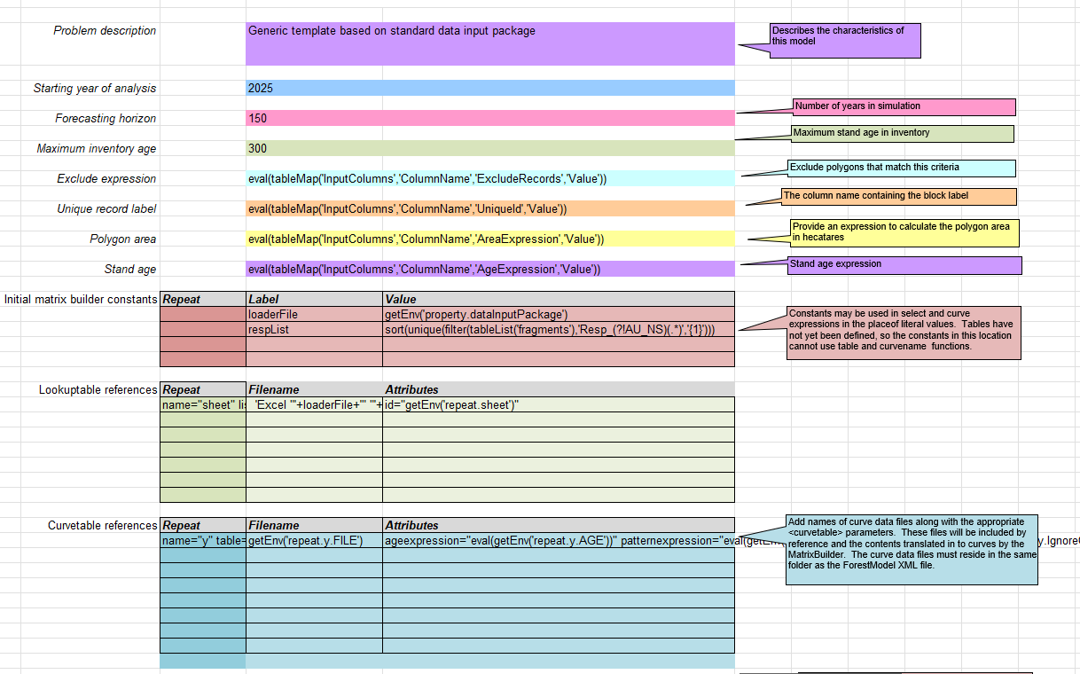
Click image to enlarge
Downloading the Ontario template
The template developed during the pilot project is available for download. The purposes for making this available are threefold. First, the data input package provides a useful outline of the key factors that should be included in a baseline forest management planning model in Ontario. Regardless of the modeling tool chosen, the relationships shown in the data input package reflect contemporary thinking about how to describe stand dynamics in Ontario. Of course, the final say in this matter rests with the planning manual and the planning team, but this data input package provides a useful starting point for that discussion.
Secondly, this code provides a complete example of a sophisticated model template. The design of this template ensures a full separation between input data and business logic. The forest specialists who will parameterize the model will work with the data input package workbook and will not require training in the complexities of the ForestModel language. Other agencies that want to take a similar approach can start by examining the architecture and implementation details of this model template.
Finally, some agencies in Ontario may want to use this model template more or less "as-is" to build their Patchworks models for the upcoming round of forest management plans. If you belong to this group, please note the following:
This template has not been 'battle tested' by being used in a plan, so it likely still contains errors and omissions. Caveat emptor; treat this model template as a draft product that requires full review and verification.
Although this template was developed during an MNR project and reviewed by MNR staff specialists, it is not an official product, and no support is provided by the MNR.
The MNR does not provide any endorsement of this template and there is no automatic guarantee that this tool will be 'blessed' for use in the upcoming round of FMPs. That is a decision to be made on a case-by-case basis by the local modeling and analysis task teams.
That being said, the template on this site may be updated when errors are noted and reported. If so, a list of changes will be recorded here along with links to the latest versions.
There are three sample data input packages available for download, one from each MNR region: Northwest (the Dog River-Matawin forest), Northeast (the Romeo Malette forest), and Southern (the French-Severn forest). Although the model template itself is small, the data input packages are quite large when you include the inventory and stand-level yield curve files. At the moment, only the data input package Excel workbook files are available for download from this site. Contact a planning specialist in your region if you would like to obtain the full package.
| Item | Date | Description |
|---|---|---|
| The model template | November 5, 2025 | The ForestModel Excel Spreadsheet that contains the model template. |
| DRM data input package | November 5, 2025 | Just the data input package Excel workbook for the Dog River-Matawin forest. This download does not include the yield curve datasets and base model inventory that are required to build the model.
This model is fairly complete and builds without error. |
| RMF data input package | November 5, 2025 | Just the data input package Excel workbook for the Romeo Malette forest. This download does not include the yield curve datasets and base model inventory that are required to build the model.
This model has incomplete succession and treatment rules that result in build errors. |
| FSF data input package | November 5, 2025 | Just the data input package Excel workbook for the French-Severn forest. This download does not include the yield curve datasets and base model inventory that are required to build the model.
This model has incomplete yield curves and succession and treatment rules that result in build errors. |